Controls from Zero

The way I was taught controls in college was flawed. Why? The method my professors used approached the topic from an aggresively mathematical background, without giving the topics a proper introduction on a fundamental level. Math is a great tool, but its only useful when you understand the premise of the problem you are trying to solve. I used to think I was “weak” in controls, but it turns out I just never learned it properly. Today, I feel much more confident on how to design and implement PID controllers. In this post, I hope to explain the fundamentals behind control systems, especially PID control systems, to those who are new to the material. Welcome to Controls from Zero.

In my hunt for information on control systems, I found a lot of resources, but there are three that I feel helped me the most, which I wanted to share.

1. Everything you need to know about control theory by Brian Douglas
2. Understanding PID Control by Brian Douglas
3. Why Laplace Transforms are useful by 3Blue1Brown

Brian Douglas’s series on MATLAB suited my learning style great, and 3Blue1Brown does a great job not just explaining how to perform a Laplace transform but also what is actually useful for, which is great.

Control Systems

A control system fundamentally just tells your machine how to behave. The best I heard it put was as a “manager for machines.” As an example, picture the HVAC system inside your house. The house is at some temperature when you modify the thermostat to 72°F. The current temperature of the house is called the state, and the value you set the thermostat to is called the reference or setpoint. Depending on the difference between the state and reference, the HVAC system will either have to heat or cool the house to get it to the desired temperature. The control system is the mathematical model that governs the HVAC system’s behavior.

There are two main categories of control systems, feedforward and feedback. Let’s start with feedforward. Imagine you have a car, and you want to maintain a speed of 60 mph. You are given a function $f(u) = x$, where $u$, the control input, is the position of the gas pedal and $x$, the control output, is the speed of the car. In this system, once you set a reference speed $r$, you can use the inverse of the function to determine what position to set the gas pedal at to maintain that speed. This is a feedforward control system, because you are not using any information about the current state of the system to determine your input. You are just using your knowledge of how the system behaves to set your input.

Feedforward control systems sound great, but there are some problems when putting them into practice. For instance, let’s say there is an extremely strong headwind while you are driving your car. This is not modeled in your function $f(u)$, so if you set your gas pedal to the position that would normally give you 60 mph, you will not actually be going 60 mph. In real life, systems tend to be unpredictable, and feedforward control systems do not handle this well. This is why feedback control systems are more commonly used.

There are multiple different type of feedback control systems. One important distinction is the difference between linear and non-linear systems. A linear system will follow the principles of what is known as superposition, which has two special properties. A nonlinear control system will not meet these specifications, and be harder to model. The two properties are:

• Homogeneity: if you increase the input by a certain factor, the output will scale by the same factor
• Additivity: if you add together two different inputs, their outputs will also be added

Another common classification of controllers is a PID controller. This is a controller with three terms added together.

• Proportional
  • $u_p(t) = K_pe(t)$
  • If there is a large error, increase the input.
• Integral
  • $u_i(t) = K_i\int_{0}^{t} e(t) \,dt$
  • This increases the input if the error has been large for a long time.
• Derivative
  • $u_d(t) = K_d\frac{d}{dt}e(t)$
  • This term reacts to the rate of change of error and helps damp oscillations.

For a PID controller, $u(t) = u_p(t) + u_i(t) + u_d(t)$.

Simulation

I have explained to you some VERY foundational topics to control systems, but there is a lot more to cover. For instance, how do you properly set the gains on a PID controller? What are some things to look out for? As part of a mini project related to this fact finding mission, I created a simulation to visualize a PID controller. This simulation allows you to change the weights and see how the resulting system behaves. All of the code is on GitHub for you to check out.

The simulation analyzes a mass spring system sliding on a flat surface. In previous iterations, I included a dampner, but to simplify the model, I ended up removing it. The system is therefore governed by the following systems of ODEs.

$v(t) = x’(t)$
$a(t) = (u(t) - kx(t)) / m$

where:

$x(t)$: position of the mass at time t
$v(t)$: velocity of the mass at time t
$a(t)$: acceleration of the mass at time t
$u(t)$: control input at time t
$k$: spring constant
$m$: mass of the object

The initial conditions for the simulation are:

$x(0) = 0$
$v(0) = 0$

The simulation makes the assumption of no friction, so the only forces acting on the mass are the spring force and the control input. The goal of the controller is to move the mass to some preset reference position r. This is one of the preset user variables. There are a couple pre-defined user variables. The first set of user variables are system variables, including:

• Mass ($m$): mass of the object
• Spring Constant ($k$): spring constant of the spring

The second set of user variables are controller variables, including:

• Proportional Gain ($K_p$): weight on the proportional term
• Integral Gain ($K_i$): weight on the integral term
• Derivative Gain ($K_d$): weight on the derivative term
• Reference Position ($r$): desired position of the mass

The third set of user variables are simulation variables, including:

• Time Step ($dt$): time step for the simulation
• Total Time ($T$): total time to simulate

Let’s try and design a controller. In the sim, we minimize independent variables by fixing mass, the spring constant, the reference position, the time step, and total time to their preset values in the simulation. In this case, those are:

$m = 1 kg$
$k = 10 N/m$
$r = 5 m$
$dt = 0.01 s$
$t = 10 s$

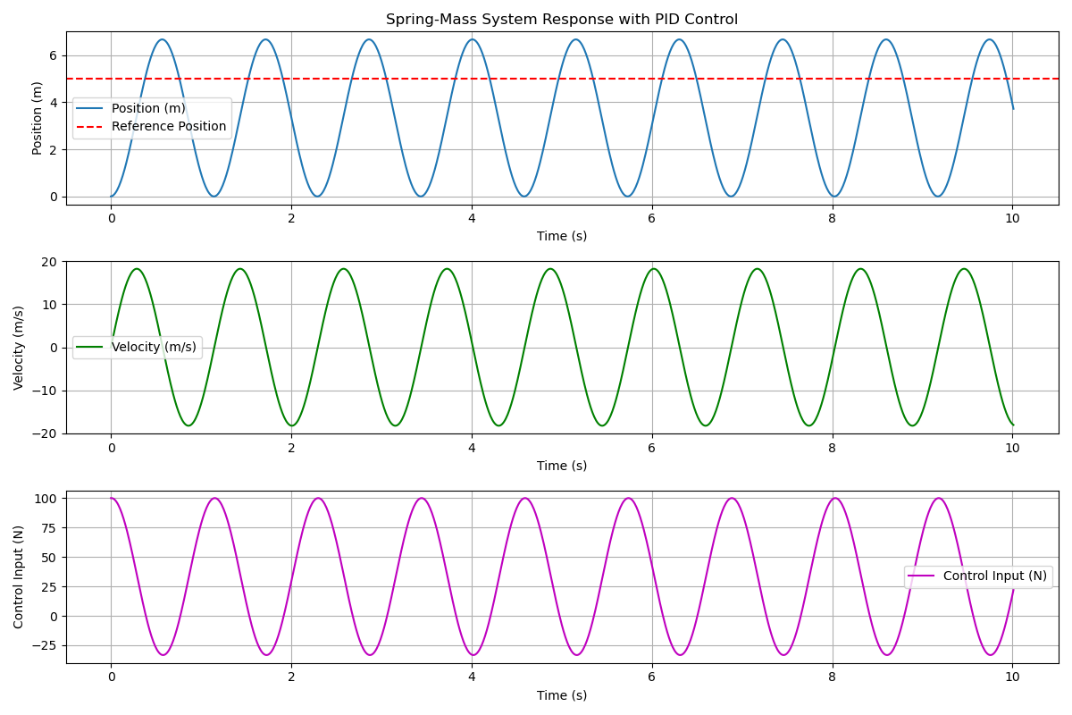
Scenario 1 ($K_p = 5, K_i = 0, K_d = 0$)

In the first scenario, we have a proportional controller with a gain of 5. Notice how we never reach our setpoint, and instead oscillate below it. This is because, at some point before reaching the setpoint, we reach a point where the spring force equals the control input. At that point, our acceleration becomes 0, and we start to decelerate. We can find this point mathematically.

$kx = K_p(r-x)$
$10x = 5(5-x)$
$15x = 25$
$x = 5/3$

This is exactly where we see the inflection point in our position graph.

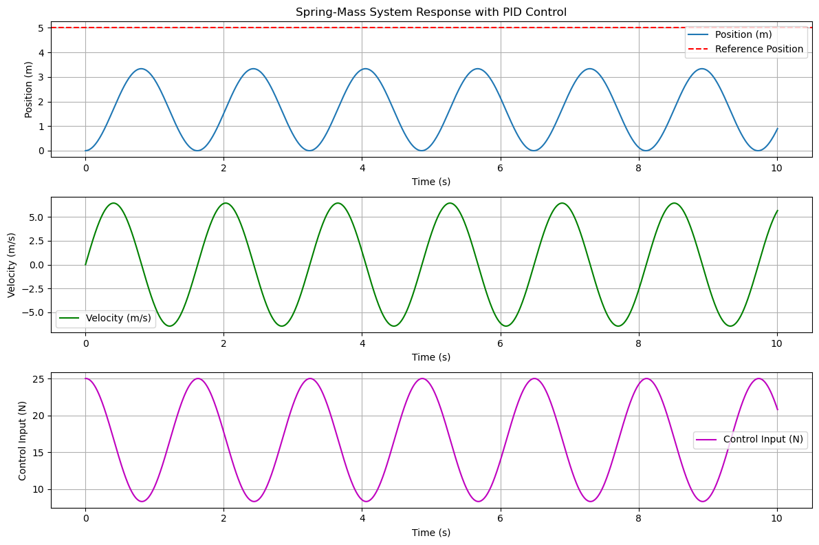
Scenario 2 ($K_p = 20, K_i = 0, K_d = 0$)

Before trying again with an integral or derivative component, I thought it would be interesting to showcase what happens with a larger proportional gain. We notice that, this time, the reference value is actually reached. With our new larger proportional gain, the point where the spring force and the control input are equal occurs at $10/3$ meters, a new, larger value. However, even after reaching the setpoint, our proportional-only controller will eventually drop again. It is clear that we need to add in some additional components to our controller to fix this.

Scenario 3 ($K_p = 20, K_i = 10, K_d = 0$)

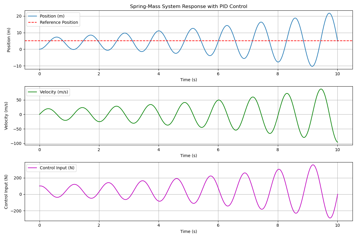
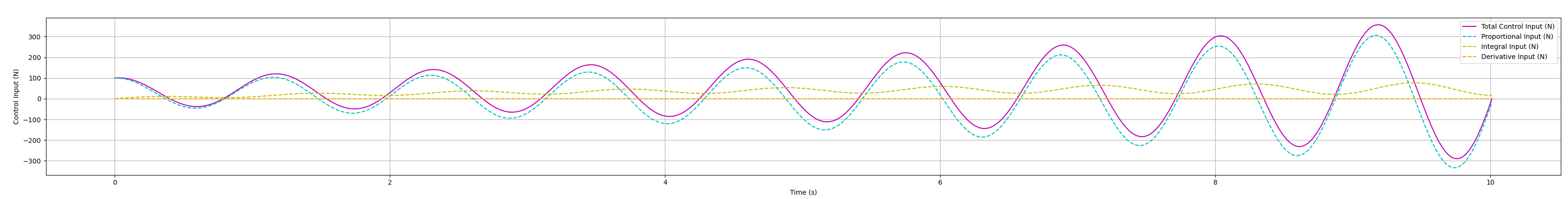
For the next scenario, we add in an integral term. Now we notice we’re diverging. It’s best to start by analyzing the behavior of the integral term we added in, and the complex interplay with the proportional term. At first, when we are below the setpoint, both the proportional and integral terms are positive. Once the setpoint is passed, the proportional term flips signs, but the integral term remains positive, due to all the positive error we have accumulated so far. It DOES start declining, but even when we cross the setpoint again, our integral input is still positive. Despite that, we enter a large dip governed by the proportional term, causing the integral term to continue to grow. This consistent growth of the integral term is what causes the divergence we see in the system. To visualize this better, I’ve broken down the individual terms below.

Scenario 4 ($K_p = 20, K_i = 10, K_d = 10$)

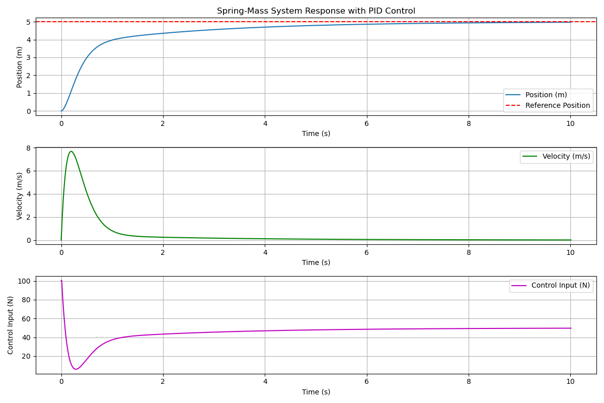
We’ve had some problems with a P and a PI controller, so let’s see if adding in a derivative term helps. In theory, the derivative term should counteract the overshoot we were seeing that caused the divergence. Looking at the results, we can see that we are now converging to the setpoint! The derivative term is doing its job of damping oscillations. However, it takes us a while to converge. Maybe we can modify the gains to get a faster response.

Scenario 5 ($K_p = 50, K_i = 30, K_d = 15$)

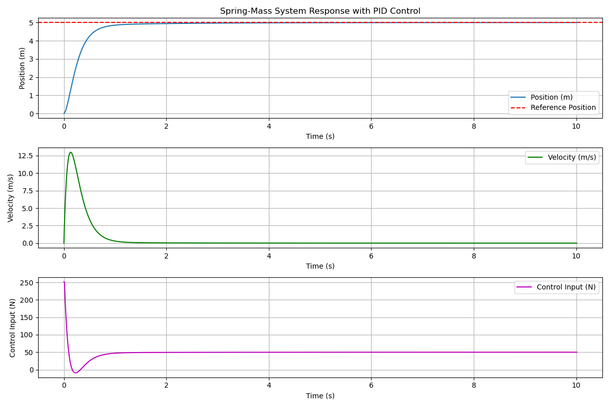
In this scenario, all of the gains are increased. The system converges much faster. It may be possible to improve this solution further, but this is a good stopping point for now.

Issues with PID Control

While PID controllers are very common and useful, they do have some problems. One classic problem is integral windup. This is a common issue in real systems due to what’s known as saturation. Imagine you have a motor, and you are using a PID controller to control its speed. The motor can only go so fast, so if your control input exceeds the maximum speed of the motor, the motor will just go at its maximum speed. This is saturation. If you then go past the setpoint, the controller will start to tell the motor to slow down, but the motors will stay at the same speed until the control input drops below the maximum speed again. This is undesirable behavior, but can be fixed with some anti-windup techniques.

Another issue is caused by the presence of high frequency noise. Imagine you have some noise described by $f(t) = A\sin(\omega t)$. The derivative of this term is $f’(t) = A\omega\cos(\omega t)$. As you can see, the derivative term is scaled by the frequency of the noise. This means that high frequency noise, even at low amplitudes, can be seen in the results. This is often fixed by adding a low-pass filter to the derivative term.

I won’t cover anti-windup techniques or filtering techniques in this post, but I may cover them in a future post. I bring it up just to show that even though PID controllers are simple in theory, they are deceptively complex in practice, and there are a lot of things that could pop up. In the future, I may cover more advanced control techniques and add more situations to the simulation, so stay tuned!